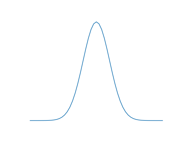
Gaussian Discriminative Analysis

The Gaussian discriminate analysis is a generative learning algorithm which models the PDF using a (multivariate) Gaussian distribution. This class of density estimation is also called parametric density estimation.

Parametric Density Estimation: To get an idea of the underlying distribution of the features we try to estimate this distribution based on a formula with parameters. Most commenly used formula for parametric density estimation is the Gaussian distribution:

1D Gaussian

\[\begin{aligned} \mathcal{N}(\mu, \sigma^{2}) = \dfrac{1}{\sigma \sqrt{2\pi}} \exp{(-\dfrac{1}{2} ( \dfrac{x-\mu}{\sigma})^{2})} \end{aligned}\]

Multivariate Gaussian

\[\begin{aligned} \mathcal{N}(\mu, \Sigma) = \dfrac{1}{(2\pi)^{n/2} |\Sigma^{1/2}| } \exp{(-\dfrac{1}{2} (x-\mu)^{T} \Sigma^{-1} (x-\mu) )} \end{aligned}\]

Quadratic discriminate analysis

Quadratic discriminate analysis is a form of GDA where the class conditional probability of each class is modeled using individual gaussians, which means that $\sigma$ of each class are not necessarily the same.

In binary (two class) QDA the classification is based on the discriminant:

\[\begin{aligned} f(x) = \text{log} \ p(y_1 | x) - \text{ log } \ p(y_2 | x) \end{aligned}\]

A positive discriminant means the posterior probability of class 1 is higher and thus we classify $x$ as class 1. The log of the posterior probabilities is taken because this yields a simpler (more efficient) equation. This is possible because log is a monotonically increasing function, which means that the relations of order are unchanged. The $max_i$ $p(y_i|x)$ will also be the $max_i$ log $p(y_i|x)$. From the log of the posterior probability follows:

\[\begin{aligned} p(y_i|x) &= \dfrac{p(x|y_i)p(y_i)}{p(x)} \\ \log{p(y_i|x)} &= \log{p(x|y_i)} + \log{p(y_i)} - \log{p(x)} \\ &= -\dfrac{p}{2}\log{2\pi} -\dfrac{1}{2}\log{\det{\Sigma_i}} - \dfrac{1}{2}(x-\mu_i)^T\Sigma_i^{-1}(x-\mu_i) \\ &+ \log{p(y_i)} - \log{p(x)} \\ \end{aligned}\]

Removing all non-class dependent constants yields:

\[\begin{aligned} \log{p(y_i|x)} &= -\dfrac{1}{2}\log{\det{\Sigma_i}} - \dfrac{1}{2}(x-\mu_i)^T\Sigma_i^{-1}(x-\mu_i) + \log{p(y_i)} \end{aligned}\]

Plugging the result into the discriminant equation yields:

\[\begin{aligned} f(x) &= \log{p(y_1|x)} - \log{p(y_2|x)} \\ f(x) &= x^T W x + w^T x + w_0 \\ W &= \dfrac{1}{2} (\Sigma_2^{-1} - \Sigma_1^{-1}) \\ w &= \mu_1^T\Sigma_1^{-1} - \mu_2^T\Sigma_2^{-1} \\ w_0 &= -\dfrac{1}{2}\log{\det{\Sigma_1}} - \dfrac{1}{2}\mu_1^T\Sigma_1^{-1}\mu_1 + \log{p(y_1)} \\ &+ \dfrac{1}{2}\log{\det{\Sigma_2}} + \dfrac{1}{2}\mu_2^T\Sigma_2^{-1}\mu_2 - \log{p(y_2)} \\ \end{aligned}\]

This is a quadratic equation modeling the decision boundary for a two class classification problem. The final class prediction or hypothesis $h(x)$ is then given by the following bernouilli distribution.

Linear discriminate analysis

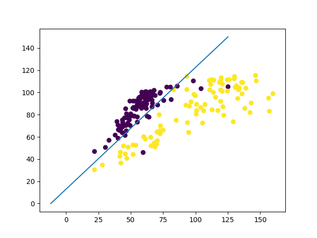
Given the assumption that the covariance matrices of both classes are equal $(\Sigma_1 == \Sigma_2)$, the decision boundary becomes linear:

\[\begin{aligned} f(x) &= w^T x + w_0 \\ w &= \hat{\Sigma}^{-1} (\hat{\mu}_2 - \hat{\mu}_1) \\ w_0 &= \dfrac{1}{2} \hat{\mu}_2^T \hat{\Sigma}^{-1} \hat{\mu}_2 - \dfrac{1}{2} \hat{\mu}_1^T \hat{\Sigma}^{-1} \hat{\mu}_1 + \log{\dfrac{p(y_1)}{p(y_2)}} \\ \end{aligned}\]

Also called Fisher's Linear Discriminate analysis.

LDA example

LDA as a dimensionality reduction technique

In Fisher's article he observes that at the decision boundary (discriminant = 0), the ratio of between and within class variance is:

\[\begin{aligned} \Phi = \dfrac{\text{variance between}}{\text{variance within}} = \dfrac{[\omega \mu_1 - \omega \mu_0]^2}{\omega^T \Sigma_1 \omega + \omega^T \Sigma_0 \omega} \end{aligned}\]

Here $\omega$ is a unit vector in a certain direction. He furthermore obeserves that this ratio is maximal for, $\omega$ as in LDA:

\[\begin{aligned} \omega &= \hat{\Sigma}^{-1} (\hat{\mu}_2 - \hat{\mu}_1) \\ \end{aligned}\]

The simple interpretation of this is that, the dicision boundary has a slope which is equal to the direction of maximum $\Phi$.

The use LDA as a dimensionality reduction technique all you have to do is map the data onto the first $k$ principal axes of the $\Phi$. (Later on we will have a look at other similar dimensionality reduction technique such as PCA)